JSX Visualization Text and Canvases

Writing text
- Appearance of variables
- IF and IFELSE
Setting up canvases
Placing canvases side-by-side

Writing text

With the text command you can write texts which explain the visualization. As value you can use LaTeX. If you want
to display a variable in the text (for example in formulas) you can use the tex-like command \var{a}.

1
2
3
4 \text{$g$ is a line that runs through $P_1 = \var{p1}$ and $P_2 = \var{p2}$} %write the content in a line
\text{The equation for the line is $\var{g}$.}       % long lines are wrapped automatically. 
\text{....} % next line
\text[c]{$y = mx + b = \var{mRes}x + \var{b}$} %write the formula in next line with center alignment

There is an optional argument that indicates the alignment of the text.
Default is l for left, but c for center and r for right alignment are also possible.

Different to the generic problem, \var{p1} will be replaced with an interactive object which might change its value if it has dependency to another variable, or even gets edited from the user if it is editable. A command \var{p1} always has to be in math mode.

Appearance of variables

You can influence the appearance of variables in text.
One command is \field which determines the number class for the variable.
Full details are given here.

IF and IFELSE

In the \text command you can use \IF{condition}{sometext} and
\IFELSE{condition}{sometext}{othertext} to write text that depends on a certain condition to hold. If the condition condition holds sometext will be shown. In case of \IFELSE, if condition does not hold, othertext is shown.
Of course, onetext or othertext can be empty.

1
2
3
4
5
6
7
8
9
10
11 \begin{visualization}{jsxviz1}
\begin{variables}
  \number[editable]{a}{1}
  \number[editable]{b}{2}
  \number{adivb}{a/b}
\end{variables}
\field{a,b,adivb}{rational}
...
\text{$\IFELSE{b=0}{\infinity}{\var{adivb}}$}
...
\end{visualization}

The condition can be a logical composition of elementary conditions:

1
2
3
4
5
6
7
8
9 \begin{visualization}{jsxviz2}
\begin{variables}
  \randint[Z]{a}{-5}{5}
  \randint[Z]{b}{-5}{5}
\end{variables}
...
\text{$\var{a}$ and $\var{b}$ have \IFELSE{[a>0 AND b>0] OR [a<0 AND b<0]}{the same signs.}{different signs.}}
...
\end{visualization}

The syntax used for condition is the same as the condition syntax of \randadjustIf. However, you can use the
values of any variable here, including e.g. coordinates of points on parametric curves.

It is also possible to combine multiple \IFELSE as in the following example

1
2
3
4
5
6
7
8
9
10
11
12
13
14
15
16
17
18 \begin{visualization}{jsxviz3}
\begin{variables}
  \number[editable]{a1}{1}
  \number[editable]{b1}{2}
  \number[editable]{c1}{3}
  \number[editable]{a2}{4}
  \number[editable]{b2}{5}
  \number[editable]{c2}{6}
\end{variables}
...
\text[c]{$\var{a1}x + \var{b1}y = \var{c1}$\\ $\var{a2}x + \var{b2}y = \var{c2}$} % display linear equation system
\text[c]{
  \IFELSE{(a1*b2) = (a2*b1)}{
     \IFELSE{(a1*c2) = (a2*c1)}{The above system of equations has an 
infinite number of solutions.}{The above system of equations has no solution.}
  }{The above system of equations has exactly one solution.}
}
\end{visualization}

Setting up canvases

The main part of the visualization is the canvas or several canvases where all or some geometric objects are plotted.
This is set up in a canvas-environment.

1
2
3
4
5
6
7
8
9
10 \begin{canvas}
  \plotSize{250,250}        % creates a 250px X 250px canvas (if the screen allows) 
  \plotLeft{-5}
  \plotRight{5}                     % initial x-axis will go from -5 to 5
  \plotBottom{-5}
  \plotTop{5}                     % initial y-axis will go from -5 to 5
  \plot[coordinateSystem]{p1,p2,g}  % plots p1, p2 and g with coordinate system
  \xAxis{$x$}            % adds the label x to the x-axis
  \yAxis{$\alpha$}           % adds the label αlpha to the y-axis
\end{canvas}

Settings of size and ranges

The size and ranges of the canvas are set with the top five commands in the previous example.

About the commands:

\plotSize{width,height}: Sets the maximal size of the canvas. If the screen is to small, the canvas
will shrink automatically,
\plotLeft and \plotRight: range for the x-axis from left to right,
\plotBottom and \plotTop: range for the y-axis from bottom to top,

All of these commands are optional, and default values or computed values will be used if not set. It is also possible to only set the
width of the canvas via \plotSize{width} instead of \plotSize{width,height}. If not all values are set other values
are chosen such that the scaling for both axis are the same.

Examples:

1
2
3
4
5
6 \begin{canvas}
  \plotSize{250,150}       
  \plotLeft{-5}
  \plotRight{5}                     
  \plot[coordinateSystem]{p1,p2,g} 
\end{canvas}

Here, we obtain a 250px x 150px canvas with x-axis going from -5 to 5. The y-axis will have the same scaling
as the x-axis, and the x-axis will be centered vertically, i.e. the y-axis will range from -3 to 3 in this case.

1
2
3
4
5
6
7
8 \begin{canvas}
  \plotSize{250}       
  \plotLeft{-5}
  \plotRight{5}                     
  \plotBottom{-3}
  \plotTop{5}
  \plot[coordinateSystem]{p1,p2,g} 
\end{canvas}

Here, we obtain a canvas with width 250px, its x-axis going from -5 to 5, and the y-axis going from
-3 to 5. The height of the canvas will be computed such that the x-axis and y-axis have the same scaling, i.e.
the height will be 200px.

Plotting objects, coordinate systems etc.

The command \plot determines what is shown on the canvas. The \plot-command has an optional argument and a mandatory
argument.

The mandatory argument is a comma separated list of the variable names that shall be shown in the canvas.
The optional argument is a comma separated list of several options. These are:

coordinateSystem: Show the coordinate system,
numberLine: Show a number line,
showPointCoords: Show the coordinates of points if you hover over them with the mouse,
noToolbar: Hide the toolbar in the canvas.

You can have multiple canvases in one visualization, and you can display the same variable in whichever canvases you like.

Labeling the axes

Within the canvas environment, you can use the commands \xAxis and \yAxis to add labels to the axes. For example, \xAxis{t} adds the label t to the x-axis.

You can use the common LaTeX-syntax for the labels. For example, if the t above should be in math mode, you write
\xAxis{$t$}.

Snap to Grid

There is one additional command that can be used in the canvas-environment. This is
\snapToGrid{xvalue,yvalue}.
This command causes all points to move to the specified grid after being dragged or
being changed in text. For example, \snapToGrid{0.5,1/3} would move the points to the nearest
spot having half-integral x-coordinate and third-integral y-coordinate.

The command \snapToGrid is especially useful in combination with problems where the answer is
taken from the graphics and one would like to minimize/avoid rounding errors.

Placing canvases side-by-side

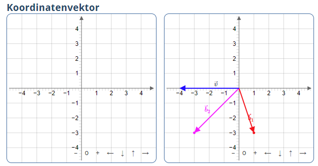
Usually, each canvas is placed in its on row. If you want to display two or more canvases next to each other, you can use the environment canvasRow. The following example illustrates the usage:

1
2
3
4
5
6
7
8
9
10
11
12
13
14
15
16
17
18
19
20
21 \begin{visualization}{viz}
    \title{Koordinatenvektor}
    ...
    \begin{canvasRow}   
        \begin{canvas}
            \plotSize{300,300}
            \plotLeft{-5}
            \plotRight{5}
            \plot[coordinateSystem]{}
          \end{canvas}
 
          \begin{canvas}
            \plotSize{300,300}
            \plotLeft{-5}
            \plotRight{5}
            \plot[coordinateSystem]{b1vec,b2vec,b1,b2,vvec,l1b1vec,l2b2vec}
            \snapToGrid{0.1,0.1}
        \end{canvas}
    \end{canvasRow}
    ... 
\end{visualization}

News