News
Index
Working with MUMIE as author
- Initial steps:
- Articles:
- Problems:
- Programming with Python
- Visualizations with JSXGraph
- Visualizations with CindyJS
- Media Documents:
Working with MUMIE as teacher
Using MUMIE via plugin in local LMS
FAQ
You're not logged in
Working with MUMIE as author
Working with MUMIE as teacher
Using MUMIE via plugin in local LMS
FAQ
At the beginning of the genericGWTVisualization you can define variables. A variable can later be used to:
12 \begin{variables}\end{variables}
Supported are random integers, doubles, and rationals.
(!) Unlike the generic problem, the random variables only exists on runtime. It will be generated every time the page is reloaded. (!)
randint
12 \randint{name}{min}{max} %creates a random integer from [min, max] and store it as name\randint[Z]{name}{min}{max} %same as above, but avoiding zero
randdouble
1 \randdouble{name}{min}{max} %creates a random real number between [min, max]
randrat
1 \randrat{name}{minNumerator}{maxNumerator}{minDenominator}{maxDenominator} %creates a random rational number with numerator from [minNumerator, maxNumerator] and denominator from [minDenominator,maxDenominator]
You can use \randadjustIf also in the variables environment of a generic visualization.
The syntax is the same as \randadjustIf in generic problems, but only random variables can be used in
the variables argument.
1 \randadjustIf{variables}{condition}
Example:
123 \randint[Z]{x1}{-5}{5}\randint[Z]{x2}{-5}{5}\randadjustIf{x1, x2}{x1 >= x2} % regenerate both x1 and x2 if x2 is not greater than x1.
This group consists of numbers, functions and geometry variables. This type of variables can also be editable by the user and be dependant on other variables.
The common syntax of the variables is:
1 \type[editable]{name}{field}{value}
i
\text{}, then the user can edit it. If you put editable points, lines and vectors on a \plot{}, users are able to drag and move them around.123456789101112131415 %simply a number\number{simple}{real}{0.5} % creates a real number with the value of 0.5\number{sipmle2}{real}{1/2} % also creates 0.5\number{simpleint}{integer}{0.5} % creates an integer with value 0%complex\number{c1}{complex}{1,-1} % creates a complex number with the value 1 - i %operation\number{op}{operation}{sin(pi)} % creates an operation sin(\pi)%using other variables\randint{randomA}{-5}{5} %create random value for a\randint{randomB}{-5}{5} %create random value for b\number[editable]{a}{integer}{var(randomA)} %creates an editable variable a with a random default value\number[editable]{b}{integer}{var(randomB)} %creates an editable variable b with a random default value\number{a+b}{operation}{var(a) + var(b)} %creates an operation a + b, where a and b will be replaced by the current value of a and b.\number{result}{integer}{var(a)+var(b)} %creates an integer with the value of a+b. The value of result will be updated everytime the user edits either a or b.
Numbers which are added to a graph can also be adjusted by a slider. To achieve this, define your number
as is done above and then use the following command inside the variables environment:
1 \slider[<step_size>]{<var_name>}{<num_var>}{<left_bound>, editable}{<right_bound>, editable}
Optional parameters (displayed in square brackets)
The slider must then be added to the graph. The syntax for this is as following:
123 \begin{canvas} \slider{<slider_var1>, <slider_var2, ...}\end{canvas}
\slider command is used to display the sliders defined in the variable environment.A simple example of the syntax
123456 \begin{variables} \number{n}{real}{-1} \slider[0.2]{n_slider}{n}{-5}{5, editable}\end{variables} \label{h}{$\textcolor{BLACK}{b =}$}
Results in the following:
with step sizes of 0.2.
Note that a slider can only be displayed in combination with a graph, see example below.
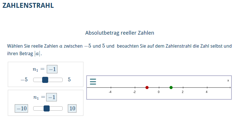
This example creates a graph which plots two points, (1) real number n and (2) absolute of number n.
Two sliders are created, both adjusting number n.
The points and the slider are then added to the canvas.
1234567891011121314151617181920212223 \title{Absolutbetrag reeller Zahlen} \text{Wählen Sie reelle Zahlen $a$ zwischen $-5$ und $5$ und beoachten Sie auf dem Zahlenstrahl die Zahl selbst und ihren Betrag $|a|$.} \begin{variables} \number[editable]{n}{real}{-1} \slider{n_s1}{n}{-5}{5} \slider[1]{n_s2}{n}{-10, editable}{10, editable} \number{absn}{real}{absn(var(n))} \point{p1}{real}{var(n),0} \point{p2}{real}{var(absn),0}\end{variables} \label{n}{$n_1 =$} \begin{canvas} \plotSize{500,80} \plotLeft{-6} \plotRight{6} \plot[numberLine]{p1,p2} \slider{n_s1, n_s2}\end{canvas}
Results in the following:
1 \function{f}{real}{sin(x)}
1234 \point[editable]{p0}{real}{0,0} % creates an editable point at 0,0\randint[Z]{a}{-3}{3}\randint[Z]{b}{-3}{3}\point[editable]{p1}{real}{var(a), var(b)} % creates an editable point with random default coordinate
Line and line segment expects you to use 2 point variables as value
12 \line{g}{real}{var(p0), var(p1)} % crates a line that runs through p0 and p1\segment{g}{real}{var(p0), var(p1)} % crates a line segment between p0 and p1
Vector is an arrow starting from the origin and ending at a point, the command expects only one point as value.
Affine vector expects as input two vectors. It is an arrow starting at the endpoint of the first vector, and being parallel to the second vector.
12345 \point{p1}{real}{1,1}\point{p2}{real}{3,0}\vector{v1}{real}{var(p1)} % creates an arrow starting from origin to (1,1)\vector{v2}{real}{var(p2)} % creates an arrow starting from origin to (3,0)\affine{aff1}{real}{var(v1),var(v2)} % creates an arrow starting from (1,1) with coordinate (3,0)
12 \point{center}{real}{1,1}\circle{c1}{real}{var(center), 2} %creates a circle on center with radius 2
12 \point{center}{real}{1,1}\angle{c1}{real}{var(center), 2, 0, pi/2} %creates an angle on center with radius 2 from 0 to pi/2
With set you can display section(s) of the 2d coordinate system (basically a set of (x,y)-tuple) that fulfills the given relation.
1 \set{set2}{real}{|var(p)x+var(q)y+var(c)|>var(d)}
Note that the value is a relation and you can combine relations with AND and OR. For example, to create a set equivalent to the above example, you can also use:
1 \set{set2}{real}{var(p)x+var(q)y+var(c)>var(d) OR -(var(p)x+var(q)y+var(c))>var(d)}
You can use the square brackets to group a part of the relation
1 \set{set2}{real}{y > 0 AND [x < -3 OR x > 3]}
\parametricFunction plots a function with one parameter (t). The value of \parametricFunction has the following arguments:
1 \parametricFunction{f}{real}{2abs(cos(2t))*cos(t)-3, 5*abs(sin(t))*sin(t)-3, 0, 2*pi, 1000}
You can add a point to the graph of a function or to the curve of a parametric function by using the commands\pointOnCurve or \pointOnParametricCurve.
\pointOnCurve has as the following arguments:
123 \function[editable]{f}{real}{sin(x)}\pointOnCurve{p}{real}{var(f)}{1}\pointOnCurve[0,2*pi]{q}{real}{cos(x)}{0}
\pointOnParametricCurve has as the following arguments:
123 \parametricFunction{f}{real}{2abs(cos(2t))*cos(t), 5*abs(sin(t))*sin(t), 0, 2*pi, 1000}\pointOnParametricCurve{p}{real}{var(f)}{0}\pointOnParametricCurve{q}{real}{cos(t), sin(t), 0, 2*pi, 1000)}{pi}
This feature is currently not supported. We intend to enhance it again in the new framework that we are currently developing.
Updated by Andreas Maurischat, 6 years ago – 297aca7