JSX Visualization Variables
Caution: The syntax for the deprecated environment \begin{genericJSXVisualization} is a bit different. Namely,
in that environment one has to provide also a "field" (real or rational) in the definition of most types.
Define variables
At the beginning of the visualization you can define variables. A variable can later be used to:
- create another variable that depends on this variable,
- be displayed in 2D-canvases or 3D-canvases (does not apply for number variables),
- be displayed in text-part as a formula, or number,
1 2 | \begin{variables}
\end{variables}
|
Random numbers
Supported are random integers, doubles, and rationals.
randint
1 2 | \randint{name}{min}{max} %creates a random integer from [min, max] and store it as name
\randint[Z]{name}{min}{max} %same as above, but avoiding zero
|
randdouble
1 | \randdouble{name}{min}{max} %creates a random real number between [min, max]
|
randrat
1 | \randrat{name}{minNumerator}{maxNumerator}{minDenominator}{maxDenominator} %creates a random rational number with numerator from [minNumerator, maxNumerator] and denominator from [minDenominator,maxDenominator]
|
Only numbers are allowed to be used as min and max value.
\randadjustIf
You can use \randadjustIf also in the variables environment of a visualization.
The syntax is the same as \randadjustIf in generic problems, and you can use almost all types of variables
in the condition argument. Exception is a coordinate of point on a parametric curve, or any variable depending on such.
1 | \randadjustIf{variables}{condition}
|
Example:
1 2 3 4 | \randint[Z]{x1}{-5}{5}
\randint[Z]{x2}{-5}{5}
\point{p}{x1^2,x1+x2}
\randadjustIf{x1, x2}{p[x]+p[y] >= 10} % redraw both x1 and x2 if the sum of the coordinates of p is at least 10.
|
Other variables
This group consists of numbers, functions and geometry variables. These types of variables can also be editable by the user and be dependant on other variables.
The common syntax of the variables is (with one exception, namely the type string ):
1 | \type[editable]{name}{value}
|
Exceptions to this syntax are variables retrieved from problems using \problem or \question
- editable is an optional argument that enables user interactivity. An editable variable can usually be edited by the user
when you use it in a \text{}, and dragged around when you put it on a \plot{}.
- name is the name of the variable to which you refer when you define other variables depending on it, when you use it in text, and
when you plot it.
- value defines the value of the variable. Here expressions are expected. Depending on the type it may
have one or more comma separated expressions. You can use other variables by using the name of that variable.
Editability
The flag editable not only affects whether the user can change the variable/element, but also its dependence behaviour on the variables which occur
in its definition.
- If a variable/element is not editable, the defining term will make the element dependent from all elements
appearing in the definition. If one of the latter is changed (by drag, text input, change of parent elements ...), the element will also change.
- If an element is editable, the defining term is used as initial value. Changing elements occurring in the
defining term will not change the editable element.
Exceptions from this behaviour:
The geometric objects lines, circles, vectors, affines, polygons, angles, and arcs are intimately linked to points occuring as defining points in its definition.
That means two things:
- Changing a point (by drag, input, change of parent) leads to changes of all these geometric objects depending on the point (even if they are
editable).
- These geometric objects can only be dragged if they are made editable AND its defining point(s) are editable. Furthermore,
these defining points must not be points on curves, as those are not freely draggable.
If the prerequisites for dragging the object are fulfilled, dragging the geometric object also moves the point(s).
- Also the elements can only be edited in text if they are made editable AND all points that would be moved by changing the value are editable, too.
Example:
1 2 3 4 5 6 | \begin{variables}
\number[edtiable]{n}{0.5} % creates a real number with value 0.5 which is editable in text,
\point{p}{n,n} % creates a non-editable point whose x-coordinate and y-coordinate both equal the number n,
\point[editable]{q}{n,-n} % creates an editable point with x-coordinate n and y-coordinate -n,
\segment[editable]{s}{p,q} % creates the segment starting at p and ending at q.
\end{variables}
|
In this example, the point _p_ is not editable. The user will neither be able to drag it in the canvas nor to change its value
in the text. However, if the user changes the value of _n_, the point will move to the new coordinates (n,n).
The point _q_ is editable, and hence the user can drag it in the canvas, and also change its value in text. Its initial
coordinates are given as (0.5,-0.5) as initially n=0.5. As _q_ is editable, however, it will not move when _n_ is changed.
Finally, the segment _s_ is intimately linked to the points _p_ and _q_. If one of the points move/are moved, _s_ changes accordingly
to stay the segment linking _p_ and _q_. Although _s_ is editable, it can not be dragged, since the point _p_ can not be dragged.
However, in text the displayed value of _s_ -- which is its length -- can be changed. In this case, the second point _q_
will be moved to fit the desired distance to _p_. If the second point wouldn't be editable, the displayed value would not be changeable.
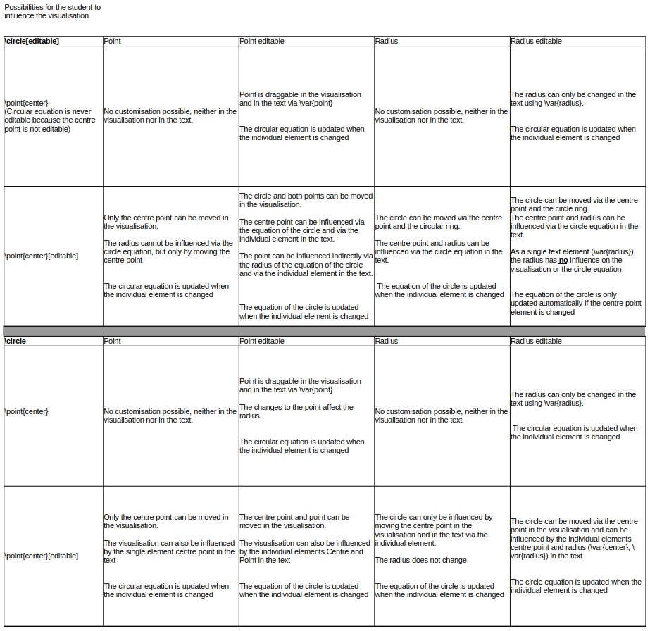
see possibilities for circle
Available types of variables
The available types of variables are number (cannot be shown in canvases), and
- displayable in 2D-canvases: function, point, line, segment, vector, affine, circle, arc, angle, polygon, parametricFunction, pointOnCurve, set, slider, string, sequence, horizontalStrip, verticalStrip, checkbox, graphNode, graphEdge
- displayable in 3D-canvases: function, point, line, segment, vector, affine, plane, polygon, sphere, curve, parametricSurface
- with special feature: onClickArrows, onClickSelect
For the types function, point etc. that are available for 2D and 3D, MUMIE will recognize from your defining input whether it is for 2D or 3D.
Numbers
1 2 3 4 5 6 7 8 9 10 11 | \begin{variables}
\number{simple}{0.5} % creates a real number with the value of 0.5
\number[editable]{simple2}{1/2} % also creates 0.5, but this time the number is editable in text
\number{simpleint}{0.5} % also would create 0.5; but by the field command below turns it into an integer with value 1 (0.5 rounded to an integer.)
\randint{randomA}{-5}{5} %creates a random value
\randint{randomB}{-5}{5} %creates a random value
\number[editable]{a}{randomA} %creates an editable number variable a with initial value randomA
\number[editable]{b}{randomB} %creates an editable number variable b with initial value randomB
\end{variables}
\field{simpleint, a}{integer} % Defines simpleint and a to always be integers
\field{b}{rational} % Defines b to be displayed as a rational fraction and not as a decimal.
|
A number variable is defined by the command \number followed by the name of the variable, and the value of the variable given as a number expression.
Function
1 2 3 4 5 6 7 | \slider{s}{2,0,4}
\function{f}{s*sin(x)}
\function[editable]{g}{sqrt(x^2+1)}
\function{h}{f*g+(1+x)}
\function{f3D}{sqrt(x^2+y^2)} % 2-variate function displayable in 3D-canvas.
\number{gAtS}{g[s]} % the value of the function g at the current position of the slider.
\function{cut}{f3D[s-2,y]} % indeterminate y is replaced by the value of s-2. This results in a 1-variate function.
|
The value of a variable of type function is a function expression containing an arbitrary number of indeterminates.
If the function contains (at most) one indeterminate, the function is flagged as being displayable in 2D, if it has two indeterminates it can be displayed in 3D-canvases. Functions in more than two indeterminates can not be displayed in canvases, but used in the definition of other objects, e.g. by evaluating one indeterminate of a trivariate function to obtain a bivariate function.
If there are more than one indeterminates, they are ordered alphabetically by default.
If you like (e.g. to use a different order or to make sure that a function is recognized for 3D), you can in addition provide the indeterminates for the function, e.g. write \function{f3D}{sqrt(x^2+y^2), [x,y]}
or \function{f}{s*sin(x), [x]}
Point
1 2 3 4 5 | \point[editable]{p0}{0,0} % creates an editable point at 0,0
\randint[Z]{a}{-3}{3}
\randint[Z]{b}{-3}{3}
\point[editable]{p1}{a, b} % creates an editable point with random default coordinates
\point{p3D}{1,1,1} % provide 3 coordinates for a point in 3D
|
You can extract the x, y, and z coordinates of a point and use it as in *value* for other variables by using `p1[x]` etc.
You can also use the coordinates in texts (see Visualization Text ).
Line and Line Segment
Line and line segment expects you to use 2 point variables (also pointOnCurve is allowed) as value
1 2 | \line[editable]{l}{p0, p1} % creates a line that runs through p0 and p1
\segment[editable]{g}{p0, p1} % creates a line segment between p0 and p1
|
Depending on whether your points are 2D-points or 3D-points, the line/segment will be available for 2D or 3D.
In text, for a 2D-line l, \var{l} shows the equation of the line in the form y=m*x+b or x=a respectively. There is no text representation of 3D-lines, yet.
For the segment (2D and 3D), its length is displayed in text.
If the flag editable is set, both the line and the segment should be draggable in canvas and changeable in text.
However, they are intimately linked to the two points. So if one point is not editable or a pointOnCurve, the line or
the segment will not be draggable.
Vector and affine vector
Vector is an arrow starting from the origin and ending at a point, the command expects only one point as value. A
vector will never be draggable. However, if set to editable, its textual representation (a vector) will be editable (if the point
is also editable).
1 2 | \point{p1}{1,1}
\vector{v1}{p1} % creates an arrow starting from origin to the point p1.
|
An affine vector is an arbitrary arrow in the plane or 3D-space. There are several possibilities for defining it. You can give
(a) two points: In this case the arrow is the connecting arrow of the points.
(b) a combination of point/vector and vector/affine: The arrow starts at the point or the endpoint of the vector and
is parallel to the vector or affine.
(c) a point or vector as well as two or three numbers: Again the arrow starts at the point or the endpoint of the vector and
has the two numbers as x-component and y-component, or the three numbers as x-, y- and z-component.
1 2 3 4 5 | \point{p1}{1,1}
\point{p2}{3,0}
\vector{v2}{p2} % creates an arrow starting from origin to (3,0)
\affine{aff1}{p1,p2} % creates an arrow starting from p1 ending at p2
\affine{aff2}{p1,v2} % creates an arrow starting from p1 parallel to v2, i.e. ending at (4,1)
|
Similar to points, you can extract the components of a vector or an affine and use it as in value for other variables by using v1[x] etc.
Matrix
The variable type matrix can be specified using Python syntax, e.g. \matrix{mat}{[ [a;b];[c;d] ]}. The individual matrix entries can be numbers and variables.
The matrix can contain any number of entries and can be passed to the answer of a question:
1 2 3 4 5 6 7 8 9 10 11 12 13 14 15 16 17 18 | \begin{variables}
\randint{a}{-3}{3}
\randint{b}{-1}{1}
\point[editable]{s}{a,b}
\number{sx}{s[x]}
\number{sy}{s[y]}
\matrix{mat}{[ [a;b];[sx;sy] ]}
\end{variables}
\vectorForm{mat}{bcolumn}
\answer{mat}{1,1} % Question 1, Answer 1. answer type has to be graphics.matrix
...
\begin{answer}
\type{graphics.matrix}
\inputAsFunction{}{studSol}
\solution{A}
\checkFuncForZero{|studSol[2,1]-A[2,1]|+|studSol[2,2]-A[2,2]|}{1}{1}{1}
\end{answer}
|
The \matrix command can only be used to transfer data to the question. A visual representation in the text of the visualisation is currently not available.
Circle and Sphere
A circle and a sphere can both be defined by its center and an expression for its radius, or by its center and a point on the circle/sphere.
1 2 3 4 5 6 7 | \number[editable]{r}{2}
\point{center}{1,1}
\point[editable]{q}{2,2}
\circle[editable]{c1}{center, r} % creates a circle around center with radius 2
\circle[editable]{c2}{center, q} % creates a circle around center through the point q
\point{p3}{1,1,1}
\sphere{s}{p3,r} % creates a sphere around p3 with radius r
|
The circle/sphere is intimately linked to its center, and also to the point on the circle/sphere if it is given. That means two things:
Although, in the example the circles/spheres are set to editable, they won't be as the center is not editable. If one drags the point q,
the circle adjusts to go through the point.
For the "editable" circle c1, however, the radius r is only used as initial data. So changing r does not change c1 here.
In text, a circle is displayed by its standard equation (x-center[x])^2+(y-center[y])^2=radius^2, and a sphere
by its standard equation (x-center[x])^2+(y-center[y])^2+(z-center[z])^2=radius^2.
Arc
There are several ways to define an arc.
- By three points: its center, the starting point of the arc, and a third point giving the direction
where the arc ends,
- The center, the starting point of the arc, and the angle.
- The center, the radius, starting angle and ending angle (both with respect to the positive x-axis).
1 2 3 4 5 6 7 8 9 10 11 | \number[editable]{r}{sqrt(2)}
\point{center}{1,1}
\point[editable]{q1}{2,2}
\point[editable]{q2}{0,2}
\number[editable]{a}{pi/2}
\number[editable]{sa}{pi/4}
\number[editable]{ea}{3*pi/4}
\arc{arc1}{center, q1, q2}
\arc{arc2}{center, q1, a}
\arc{arc3}{center, r, sa,ea}
|
All three arcs in this example are the same at initialization, but of course are updated differently.
Even if set editable, an arc can only be dragged, if it is defined by three freely draggable points.
In text the arc is shown in the form
[ center[x], center[y] ] + radius * [ cos(phi),sin(phi)], startingAngle <= phi <= endingAngle
This textual representation has input fields, if the arc is editable and all points involved in the definition
(i.e. all three in the first case, two in the second case and the center in the third case) are freely draggable points.
Angle
The data to define an angle are the same, as for arc. In the case of three points, however, one
can provide an additional scaling factor to change the default size of the drawn angle.
In text the size of the angle is shown. This size can also be used to define other variables.
1 2 3 4 5 6 7 8 9 10 11 | \number[editable]{r}{sqrt(2)}
\point{center}{1,1}
\point[editable]{q1}{2,2}
\point[editable]{q2}{0,2}
\number[editable]{a}{pi/2}
\number[editable]{sa}{pi/4}
\number[editable]{ea}{3*pi/4}
\angle{angle1}{center, q1, q2, 1.3}
\angle{angle2}{center, q1, angle1}
\angle{angle3}{center, r, sa,ea}
|
All three angle variables describe the same angle in the visualization, but are shown in different sizes of radius.
Polygon
For defining a polygon, you use the command \polygon{name}{value}. The value in its definition has to be a comma separated list of points.
In text the (oriented) area of the polygon is shown. For editability, the rules explained above apply.
Polygons in 3D-space only work properly if its vertices lie in a common plane.
1 2 3 4 | \point{p1}{0,0}
\point{p2}{2,1}
\point{p3}{1,2}
\polygon{poly}{p1,p2,p3}
|
Parametric Function
The command \parametricFunction{name}{value} plots a function in 2D with one parameter. The value of \parametricFunction has the following arguments (separated by commas):
- fx - the expression defining the x component
- fy - the expression defining the y component
- min - the lower bound of the parameter
- max - the upper bound of the parameter
1 | \parametricFunction{f}{2*abs(cos(2t))*cos(t)-3, 5*abs(sin(t))*sin(t)-3, 0, 2*pi}
|
The expressions _fx_ and _fy_ are function expressions as for function explained above, and min and max are expressions determining a number as for number.
If the parametric function is non-editable, even the lower and upper bounds are updated when the variables
in their definition change.
Point on Curve
In 2D, you can add a point to the graph of a function or to the curve of a parametric function by using the command
\pointOnCurve{name}{value}. It can then only be dragged on the curve. The value-argument of the command consists of the
name of the (parametric) curve, and the initial value for the parameter or x-value, respectively.
1 2 3 4 | \function[editable]{f}{sin(x)}
\parametricFunction{g}{2*abs(cos(2t))*cos(t), 5*abs(sin(t))*sin(t), 0, 2*pi}
\pointOnCurve{p}{f,1}
\pointOnCurve{q}{g,0}
|
In the example, the point p has initial coordinates (1,sin(1)), the point q has
initial coordinates 2*(abs(cos(2*0))*cos(0), 5*abs(sin(0))*sin(0) )=(2,0).
There is no editable-flag for pointOnCurve. The point in the canvas will be always draggable, but non-editable in the text.
As it is not freely draggable in the plane, inherited behaviour of other objects (lines, vectors, polygons etc.) depending on the point
will be as if the point is not editable.
If you would like to have a point `p2` on the curve `f` which is not draggable, but moves with e.g. some slider `s`, you
should define it as \point{p2}{s,f[s]} using the syntax for evaluations of functions.
Set
With set you can display section(s) of the 2d coordinate system (basically a set of (x,y)-tuple) that fulfills the given relation.
1 2 3 | \number[editable]{p}{1}
\number[editable]{q}{-1}
\set{s}{|p*x+q*y|<sqrt(2)}
|
The value in the definition is a relation expression involving the indeterminates x and y.
You can use variables as for number and function expressions, and you can combine relations with AND and OR, and negate them
with NOT.
For example, to create a set equivalent to the above example, you can also use:
1 | \set{s2}{p*x+q*y<sqrt(2) AND p*x+q*y>-sqrt(2)}
|
You can use the square brackets or parenthesis to group a part of the relation
1 | \set{s3}{y > 0 AND [x < -3 OR x > 3]}
|
Caution: The current implementation of set is quite slow, on initialization as well as on updates.
However, if you define it to be _editable_, only the performance issue on initialization remains.
Sliders
For sliders the optional argument (usual reserved for editability) provides a step size for the values, and
the last mandatory argument (the "value" of the command) consists of a list of three expressions determining numbers,
namely the initial value of the slider, the lower bound, and the upper bound.
1 | \slider[stepsize]{name}{initialvalue,lowerbound,upperbound}
|
stepsize can be any expression determining a number. If omitted the values of the slider can change continuously.
All arguments stepsize , leftbound, rightbound will be fixed and not editable.
If named in the \plot-command of a canvas, the slider will be added to the canvas in the lower left corner
(or above other sliders if several are shown). If used in text, the current slider value will be shown
as an editable number. Sliders can not be displayed in 3D-canvases.
1 2 | \slider{s}{2,0,4}
\function{f}{s*sin(x)}
|
In this example, the slider can be used to manipulate the function f.
Text in the 2D-Canvas
With the command \string, you can define a text variable. The syntax differs from the usual one, and is
1 | \string[editable]{name}{text}{position}
|
This allows to place simple text (given in text) at the specified position in the canvas.
The additional argument position has to be given as two number expressions separated by comma.
1 | \string{mytext}{Some text}{-1,1}
|
The example provides the text "Some text" starting at the point (-1,1). Of course, you have to
add the variable name mytext to the list in the \plot-command, in order to be displayed.
Sequences
The command \sequence allows to visualize sequences. The syntax is
1 | \sequence[editable, format]{name}{value}
|
So in the optional argument, you can not only determine whether the sequence is editable or not, but also whether
it is given 'explicit' (default) or 'recursive'.
The value consists of a comma separated list of
- The start index for the sequence (given by a number expression),
- The function term for defining the
n-th value of the sequence (same rules apply as for functions).
In case of a recursive sequence with name s you refer to the previous values using s[n-1], s[n-2] etc.
- (only in case 'recursive') further number expressions defining the initial values of your recursive sequence.
Example:
1 2 3 4 | \sequence[recursive]{Fib}{1,Fib[n-1]+Fib[n-2],1,1}
\number{goldenRatio}{(1+sqrt(5))/2}
\number{conj}{1-goldenRatio}
\sequence{Fib2}{1,1/sqrt(5)*(goldenRatio^n-conj^n)}
|
The first sequence is the Fibonacci sequence in its usual recursive form.
The second is also the Fibonacci sequence in its well-known explicit form
using the golden ratio and its conjugate.
The points of a sequence can be colored in different colors depending on certain conditions.
See Coloring the points of sequences.
Horizontal and Vertical Strips
With the command \horizontalStrip and \verticalStrip, you can visualize ranges
around values on the x-axis or y-axis. The syntax is the usual one
1 | \horizontalStrip[editable]{name}{value}
|
and
1 | \verticalStrip[editable]{name}{value}
|
For example
1 | \horizontalStrip{s}{1, 0.2, >0}
|
will be displayed in the canvas as the set of all points whose y-coordinate differs
from 1 by at most 0.2, and whose x-coordinate is bigger than 0.
In detail, the value consists of a comma separated list of two or three arguments.
For \horizontalStrip, these are
- a number expression which determines the y-coordinate around which the strip is build
- a number expression which determines the width of the strip,
- optionally an expression starting with '>' or '<' followed by a number expression.
Which means that the strip starts at the number (case '>') or ends at this number (case '<').
If no third argument is given, the strip will go to infinity in both directions.
For verticalStrip, the roles of the x-coordinate and y-coordinate are just swapped.
Creating Arrows on Click
With the command \onClickArrows, you can let the user create arrows by clicking at two points, one after another.
The user can remove the arrows by clicking on them again.
You can provide a set of points eligible as source points as well as a set of points eligible as target points for the arrows,
and also give a maximum number of arrows that the user can create.
Furthermore, you can provide two set of arrows that are already shown on initialization. One set which are fixed, and cannot be removed by the user, the other which can be removed.
The syntax is the usual one
1 | \onClickArrows{name}{value}
|
where the value consists of a comma separated list of
- the list of point names eligible as source points for the arrows,
- the list of point names eligible as target points for the arrows,
- the maximum number of arrows to be created,
- the list of arrows that are there from the start, and can not be removed,
- the list of arrows that are there from the start, and can be removed.
If a list in 1. or 2. is empty (or not given at all), all points visible on the canvas are eligible.
If the maximum number of arrows is not given, the number of arrows is not limited.
The fixed arrows are not counted in the maximum number of arrows, but the non-fixed ones are.
Example:
1 2 3 4 5 | \point{p1}{1,1}
\point{p2}{1,2}
\point{q1}{2,1}
\point{q2}{2,2}
\onClickArrows{a}{[p1,p2],,4,[ [q1,p1],[q2,p2] ],}
|
Here the value consists of
- the list [p1,p2],
- an empty list,
- the number 4,
- the list of pairs [ [q1,p1],[q2,p2] ], i.e. each arrow is given by an ordered pair of points,
Hence, two arrows, one from q1 to p1 and one from q2 to p2 are shown from the start, and cannot be removed.
The user can create up to 4 arrows. The source points for these arrows are limited to p1 and p2, but the
target points are arbitrary.
For evaluating which arrows are created by the user, there are several functions/attributes available.
These functions can be used in the definition of other variables, or conditions for IFELSE and have their meaning from
regarding the arrows as describing an assignment from the set of points of possible sources to the set of
points of possible targets. The fixed arrows are taken into account for these functions.
- isMap: Result is 1, if the arrows describe a map, otherwise 0,
- injective or inj: Result is 1, if in addition the map is injective,
- surjective or surj: Result is 1, if the arrows describe a surjective map,
- bijective or bij: Result is 1, if the arrows describe a bijective map,
- numberOfArrows: the number of total arrows (fixed and non-fixed) visible,
- numberOfSources: the number of points which are actually source points of arrows,
- numberOfTargets: the number of points which are actually target points of arrows,
- hasArrow(p,q): Result is 1, if there is an arrow from the point p to the point q, otherwise 0,
- hasSource(p): Result is 1, if there is an arrow with source p, otherwise 0,
- hasTarget(q): Result is 1, if there is an arrow with target q, otherwise 0,
Example for using them:
1 2 3 4 5 6 7 8 9 10 | \begin{variables}
\point{p1}{1,1}
\point{p2}{1,2}
\point{q1}{2,1}
\point{q2}{2,2}
\onClickArrows{a}{[p1,p2],,4,[ [q1,p1], [q2,p2] ],}
\number{h}{a[hasTarget(q1)]*a[hasTarget(q2)]}
\end{variables}
\text{\IFELSE{a[isMap]=1}{The arrows represent a map.}{The arrows don't represent a map.}}
\text{\IFELSE{h=1}{Both points, q1 and q2 are targets.}{At least one of the points q1 and q2 are not targets.}}
|
Checkbox
The command \checkbox allows to add a checkbox. The syntax is
- first parameter is the name of the variable
- second parameter determines whether the checkbox is initially selected {1} or not {0}
Subsequently, the value can be used like a number variable and the checkbox can be styled like other variables, too.
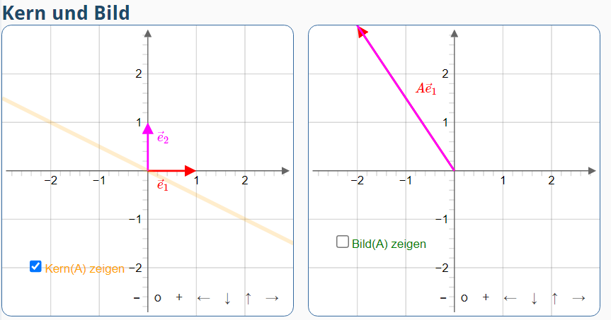
1 2 3 4 5 6 7 8 9 10 11 12 13 14 15 16 17 18 19 20 21 22 23 24 25 26 27 28 29 30 31 | \begin{visualization}[550][650]{viz}
\title{Kern und Bild}
\begin{variables}
...
\checkbox{kernToggle}{1}
\checkbox{bildToggle}{0}
...
\number{hideKern0D}{dirac(detA*kernToggle)
\number{hideBild2D}{dirac(detA*bildToggle)}
...
\end{variables}
...
\label{kernToggle}{Kern(A) zeigen}
\label{bildToggle}{Bild(A) zeigen}
...
\color{kernToggle}{orange}
\color{bildToggle}{green}
...
\begin{canvasRow}
\begin{canvas}
...
\plot[coordinateSystem]{...,kernToggle}
\end{canvas}
\begin{canvas}
...
\plot[coordinateSystem]{...,bildToggle}
\end{canvas}
\end{canvasRow}
...
\end{visualization}
|
Selecting objects
Using the command \onClickSelect, one can let the user select objects that are visible on the canvas.
The information which objects are selected can then be used in definitions of other variables.
The syntax is
1 | \onClickSelect{name}{value}
|
The value consists of a comma separated list of variable names, naming the objects that are allowed to be selected.
Optionally, one can append to this list a second list (this one enclosed in square brackets) of those objects which should be preselected.
E.g. if p and q are such objects, value could be p,q,[p] meaning that p and q can be selected and p is already preselected.
By setting a style for the onClickSelect-variable, you can define how the appearance of the objects change, when they are selected, e.g. if
the objects to be selected are points, and they should appear green, you can use
\style{sel}{fillcolor: 'green', strokecolor: 'green'} or just \style{sel}{color: 'green'}.
Here sel is the name of the onClickSelect-variable.
For accessing the information whether an object p is selected, you can use sel[p] in the definition of other variables. See the example below.
1 2 3 4 5 6 7 8 9 10 11 12 13 14 15 16 17 18 19 20 21 22 23 24 25 26 27 28 | \begin{visualization}{viz}
\title{Select the right point}
\begin{variables}
\point{p1}{1,1}
\point{p2}{1,-1}
\onClickSelect{sel}{p1,p2}
\number{p1Selected}{sel[p1]} % is 1 if p1 is selected and 0 otherwise
\number{p2Selected}{sel[p2]} % is 1 if p2 is selected and 0 otherwise
\number{n}{sel} % stores the number of currently selected objects
\end{variables}
\style{sel}{fillcolor: 'green'}
\begin{canvas}
\plotSize{300}
\plotLeft{-3}
\plotRight{3}
\plot[coordinateSystem]{p1,p2,sel}
\end{canvas}
\text{Click on the point that lies in the first quadrant.}
\text{\IFELSE{n=0}{You didn't select any point yet.}{
\IFELSE{n=2}{You selected both points.}{
\IFELSE{p1Selected}{Yes. This point is in the first quadrant.}{
No. This point is not in the first quadrant.
}
}
}
}
\end{visualization}
|
Directed Graphs
Using the commands \graphNode and \graphEdge, one can design directed graphs.
The syntax is
1 2 | \graphNode{name}{value}
\graphEdge{name}{value}
|
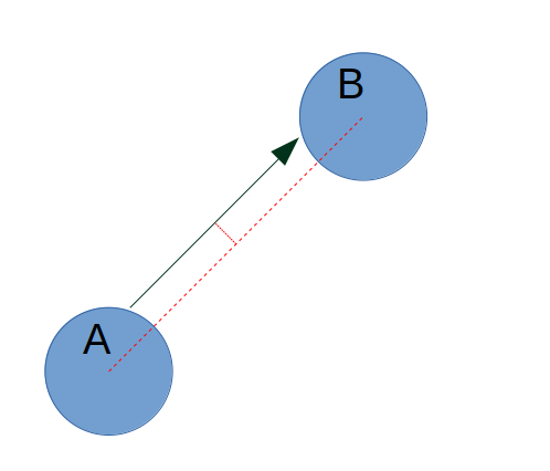
where the value of a graph node consists of two number expressions determining the position of the node (of course the two expressions are separated by comma). The value of a graph edge consists of a list of 2 up to 4 arguments:
- the name of the source node
- the name of the target node
- (optional) a weight for the edge. This weight is displayed if the edge variable is used in text.
- (optional) a number determining whether/how far the arrow is moved orthogonally to the direct line between the center of the nodes (see image).
As for (most) other variable types, for both graphNodes and graphEdges one can provide an optional argument editable by which a graph node can be dragged and the weight of the edge can be changed in text, respectively.
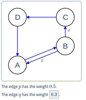
Example (source code to the directed graph above):
1 2 3 4 5 6 7 8 9 10 11 12 13 14 15 16 17 18 19 20 21 22 23 24 25 26 27 28 29 30 | \begin{visualization}{vis}
\begin{variables}
\graphNode[editable]{P1}{0,0}
\graphNode[editable]{P2}{3,1.2}
\graphNode{P3}{3,3}
\graphNode{P4}{0,3}
\graphEdge{e1}{P1,P2,,8}
\graphEdge{e1r}{P2,P1,0.5,8}
\graphEdge[editable]{e2}{P2,P3,0.3}
\graphEdge{e3}{P3,P4}
\graphEdge{e4}{P4,P1}
\end{variables}
\label{P1}{A}
\label{P2}{B}
\label{P3}{C}
\label{P4}{D}
\label{e1r}{$p$}
\label{e2}{$q$}
\begin{canvas}
\plotSize{320}
\plotLeft{-1}
\plotRight{4}
\plotBottom{-1}
\plot[noToolbar]{P1,P2,P3,P4,e1,e2,e3,e4,e1r}
\end{canvas}
\text{The edge $p$ has the weight $\var{e1r}$.\\ The edge $q$ has the weight $\var{e2}$.}
\end{visualization}
|
Internally, graph nodes are points with default styling, and graph edges are arrows. So if you want to change their appearance you can use the same styling commands as for those.
Plane
The syntax for planes is the usual one \plane{name}{value}.
However, there are several options how you define the plane:
- three points in 3D-space: the plane containing these points,
- a point and two vectors: the plane through the point in the direction given by the vectors,
- a point and a vector: the plane through the point with the given vector as normal vector.
Curve in 3D
For curves in 3D, the command is \curve{name}{value}.
Quite analogous to parametric functions in 2D, the value consists of
- fx - the expression defining the x component
- fy - the expression defining the y component
- fz - the expression defining the z component
- min - the lower bound of the parameter
- max - the upper bound of the parameter
1 | \curve{f}{2*abs(cos(2t))*cos(t)-3, 5*abs(sin(t))*sin(t)-3, t, 0, 2*pi}
|
The expressions _fx_, _fy_, and _fz_ are function expressions as for function explained above, and min and max are expressions determining a number as explained below.
If the curve is non-editable, even the lower and upper bounds are updated when the variables
in their definition change.
Parametric Surface
The command for parametric surfaces is \parametricSurface.
Its value consists of
- fx - the expression defining the x component
- fy - the expression defining the y component
- fz - the expression defining the z component
- range1 - a pair for the bounds of the first parameter
- range2 - a pair for the bounds of the second parameter
1 | \parametricSurface{f}{u+v, u*v, (u-v)^2, [0, 2], [0,2]}
|
The expressions _fx_, _fy_, and _fz_ are function expressions in two indeterminates, and range1 and range2 are pairs of expressions
determining numbers as explained below.
If the parametric surface is non-editable, even the lower and upper bounds are updated when the variables
in their definition change.
Vectorfield
The command for vector fields is \vectorfield.
In 2D, its value consists of
- fx - the expression defining the x component
- fy - the expression defining the y component
- [hl,hs,hu] - a triple for the horizontal direction determining a) the lower bound, b) the number of shown steps (=number of arrows -1), and c) the upper bound
- [vl,vs,vu] - a triple for the vertical direction determining a) the lower bound, b) the number of shown steps (=number of arrows -1), and c) the upper bound
- (optional) scaling - a number expression to change the scaling of the length of the shown vectors in the canvas (default is 1)
1 | \vectorfield{v}{2*x*y, x^2, [-2.1, 10, 2.1], [-2.1,10, 2.1]}
|
The expressions _fx_, and _fy_ are function expressions in two indeterminates, and [hl,hs,hu], and [vl,vs,vu] are triples of expressions
determining numbers as explained below.
If the vector field is non-editable, even the lower and upper bounds, and the number of steps are updated when the variables
in their definition change.
In 3D, its value consists of
- fx - the expression defining the x component
- fy - the expression defining the y component
- fz - the expression defining the z component
- [xl,xs,xu] - a triple for the direction x determining a) the lower bound, b) the number of shown steps (=number of arrows -1), and c) the upper bound
- [yl,ys,yu] - a triple for the direction y determining a) the lower bound, b) the number of shown steps (=number of arrows -1), and c) the upper bound
- [zl,zs,zu] - a triple for the direction z determining a) the lower bound, b) the number of shown steps (=number of arrows -1), and c) the upper bound
- (optional) scaling - a number expression to change the scaling of the length of the shown vectors in the canvas (default is 1)
1 | \vectorfield{v}{2*x*y, x^2+z^3,3*y*z^2, [-2.1, 10, 2.1], [-2.1,10, 2.1], [-2.1,10, 2.1]}
|
The expressions _fx_, _fy_, and _fz_ are function expressions in three indeterminates, and [xl,xs,xu], [yl,ys,yu], and [zl,zs,zu] are triples of expressions
determining numbers as explained below.
If the vector field is non-editable, even the lower and upper bounds, and the number of steps are updated when the variables in their definition change.
You can also use a variable of type vectorfield in text with the \var{..}-command. A vector containing the function terms _fx_, and _fy_ (and _fz_) is shown. The entries are editable, if you defined the variable to be editable. You can also change the appearence of the vector with the command \vectorForm{..}{..}.
Number expressions and function expressions
In visualizations, a number expression is a mathematical expression that evaluates in a number. A function expression is a mathematical expression that contains at most two indeterminates.
You can use all of the math functions abs, acos, acosh, asin, asinh, atan, atanh, cbrt, ceil, clz32, cos, cosh, exp, floor, ln, log, log10, log1p, log2, sign, sin, sinh, sqrt, tan, tanh, trunc,
as well as number values and coordinates of points/vectors defined earlier.
Evaluations and subtitutions
You can use evaluations/substitutions of functions in the value for other variables by using e.g. f[1] or f[a+1] for a function variable f and a number or function variable a.
For multivariate functions, you also have to provide the indeterminate that you would like to replace, e.g. write \function{fsub}{f3D[s-2,y]} to replace the indeterminate by the value of s-2.
You can even replace several indeterminates in one call, e.g. f[2,x][1,y].
Derivatives
Given a function variable f having an indeterminate x, you can use its derivative in expressions with the syntax D[f,x] that you are used to from expressions in the corrector of problems.
Caution
Iterated brackets are not allowed, i.e. f[p[x]] is not valid neither is f[g[0]].
In such cases, define a new variable first whose value is p[x] or g[0], respectively.
Same holds for derivatives, e.g. D[D[f,x],x] as well as D[f[2,y],x] are not valid.
Also concatenating derivatives with substitutions (e.g. D[f,x][2,x]) is not allowed, and must be split by defining a function variable with value D[f,x].