News
Index
Working with MUMIE as author
- Initial steps:
- Articles:
- Problems:
- Programming with Python
- Visualizations with JSXGraph
- Visualizations with CindyJS
- Media Documents:
Working with MUMIE as teacher
Using MUMIE via plugin in local LMS
FAQ
You're not logged in
Working with MUMIE as author
Working with MUMIE as teacher
Using MUMIE via plugin in local LMS
FAQ
For visualizations there are two environments available:\begin{visualization}... \end{visualization} as well as\begin{jsxgraph}... \end{jsxgraph}.
Both are using JSXGraph developed at the University of Bayreuth.
The former environment is more comfortable to the user as the code is written in LaTeX-style.
It can also be used in combination with problems. This means, the visualization can fetch values of number and function variables from the problem, and pass values of number and function variables to the problem as solutions to answers of type graphics.number and graphics.function.
In the environment \begin{jsxgraph}... \end{jsxgraph}, you can use actual javascript-code to create custom visualizations with the jsxgraph package.
There is also an environment \begin{genericJSXVisualization}... \end{genericJSXVisualization} which has the same behaviour as \begin{visualization}... \end{visualization}, but different syntax for defining variables.
It still works, but is deprecated.
Before starting with any visualization, make sure that the package mumie.genericvisualization or the package mumie.genericproblem are loaded in your document by inserting a line (e.g. right after \begin{content})
1 \usepackage{mumie.genericvisualization}
or
1 \usepackage{mumie.genericproblem}
Without one of these packages, generic visualizations don't work.
Example:
12345678910111213141516171819202122232425262728293031 \begin{visualizationwrapper}......\begin{visualization}{jsxviz} \title{Coordinates of a point} \begin{variables} \point[editable]{p1}{1,0} % the point can be dragged as it is set to editable. \number{px}{p1[x]} \number{py}{p1[y]} \end{variables} \label{p1}{P} \color{p1}{DARKRED} \text{In der Grafik sehen sie den Punkt $P=\var{p1}$.} \begin{canvas} \plotSize{200,200} \plotLeft{-10} \plotRight{10} \plot[coordinateSystem,showPointCoords]{p1} \end{canvas} \text{Die $x$-Koordinaten des Punktes ist $\var{px}$,\\ die $y$-Koordinate ist $\var{py}$.} \end{visualization} ......\end{visualizationwrapper}
The visualization environment starts with \begin{visualization}{_id_} and ends with \end{visualization} where you can choose any string as _id_.
For enabling visualizations, they must lie in an environment \begin{visualizationwrapper},\end{visualizationwrapper}.
However, there is only one wrapper for all visualizations of an article, and arbitrary text components of articles can also be inside this environment.
The components of the visualization are:
\title{...},\begin{variables} and \end{variables},\text{...},\begin{canvas} and \end{canvas} for 2D-canvases and between \begin{canvasXYZ} and \end{canvasXYZ} for 3D-canvases.The order in which the text-blocks and canvases appear in the code determines the order in which they are shown later.
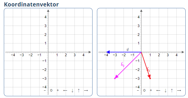
Two or more canvases can be displayed next to each other by using the canvasRow environment.
1234567891011121314151617181920 \begin{visualization}{viz} ... \begin{canvasRow} \begin{canvas} \plotSize{300,300} \plotLeft{-5} \plotRight{5} \plot[coordinateSystem]{vbvec} \end{canvas} \begin{canvas} \plotSize{300,300} \plotLeft{-5} \plotRight{5} \plot[coordinateSystem]{b1vec,b2vec,b1,b2,vvec,l1b1vec,l2b2vec} \snapToGrid{0.1,0.1} \end{canvas} \end{canvasRow} ... \end{visualization}

In addition, there are environments tabs and incremental available.
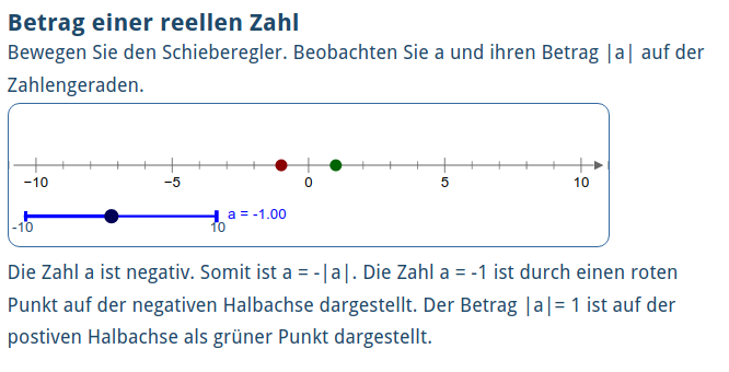
The following example illustrates how it works. More details are given later.
123456789101112131415161718192021222324252627282930313233343536 \begin{visualization}{viz} \title{Betrag einer reellen Zahl} \begin{variables} \slider{s}{-1,-10,10} % slider with name s, initial value -1 and range [-10,10] \number{a}{s} % a number with name a and same value as s. \number{b}{|a|} % a number with name b and value equal to |a|. \point{p1}{a,0} % non-editable point p1 on the x-axis with x-coordinate equal to a \point{p2}{b,0} % non-editable point p1 on the x-axis with x-coordinate equal to b \end{variables} \field{a,b}{rational} % the numbers a and b should be displayed in text as rational fractions. \label{s}{a} \color{p1}{DARKRED} \color{p2}{DARKGREEN} \text{Bewegen Sie den Schieberegler. Beobachten Sie $a$ und ihren Betrag $|a|$ auf der Zahlengeraden.} \begin{canvas} \plotSize{500,120} \plotLeft{-11} \plotRight{11} \plotBottom{-3} \plot[numberLine, noToolbar]{p1,p2,s} \end{canvas} \text{ \IFELSE{s >= 0}{ Die Zahl $a$ is positiv oder Null. Somit ist $a=|a|$ und auf der Zahlengeraden durch einen grünen Punkt dargestellt. }{ Die Zahl $a$ ist negativ. Somit ist $a = -|a|$. Die Zahl $a = \var{a}$ ist durch einen roten Punkt auf der negativen Halbachse dargestellt. Der Betrag $|a|=\var{b}$ ist auf der postiven Halbachse als grüner Punkt dargestellt. } } \end{visualization}

In the variables environment, there are five variables. The numbers and the points can not be changed directly, as the optional editable flag is not set. However, when the value of the slider is changed the values of the other variables adjust accordingly.
The label-command \label{s}{a} causes that a=-1.00 is displayed next to the slider, and the color-commands change the default colors of the points _p1_ and _p2_.
Tip: Let's say your label is a formula like x^2 and you would like that it is rendered as a math formula instead of plain text. You can achieve that with the usual LaTeX syntax: \label{s}{$x^2$}
About the commands in the canvas environment:
\plotSize determines the maximum size of the canvas in pixel (it is shrinked if the screen is too small),\plotLeft and \plotRight determine the lower and upper bound of the x-axis,\plotBottom determines the lower bound of the y-axis (the upper bound is then computed to fit),\plot determines which variables are displayed in the canvas (here _p1_, _p2_ and _s_), as well as sets some attributes. In this case, that a number line is shown and that the toolbar is hidden.The final text part contains an if-clause which shows either the first part or the second part depending on whether the value of the slider _s_ is greater or equal to zero or not.
Under the following links you get detailed information on how to create different parts of the visualization content.
Visualizations can be used with problems, too.
The syntax of the visualization is the same as when used in articles.
However, there are some additional commands so that the visualization can interact with the problem.
The visualizations will be defined outside of the problem environment, but you can make them be displayed inside question text
and explanations at the place of your choice.
In the visualization you can use the variable-types question and problem with syntax:\question{questionnr}{varname} and \problem{varname}.
The visualization then fetches the value of the variable varname from the specified question or problem, and you can use that variable as any other variable.
The questionnr in \question{questionnr}{varname} is the number of the question in your tex-document, regardless whether you are using randomquestionpools or not.
There are some restrictions/issues that you have to take into account:
editable-flag to make the variable editable in text,\question[editable]{questionnr}{varname}.Example:
1234567891011121314151617181920212223242526272829303132333435363738394041424344454647484950515253545556 \usepackage{mumie.genericproblem}\begin{visualizationwrapper}\begin{visualization}{myvisualization} \begin{variables} \question{1}{f} % the variable f will be fetched from question 1 \end{variables} \begin{canvas} \plotSize{250,250} \plotLeft{-4} \plotRight{4} \plot[coordinateSystem]{f} \end{canvas} \end{visualization} \end{visualizationwrapper} \begin{problem} \begin{variables} \randint{c}{1}{3} % integer in the range [-3,3] \begin{switch} \begin{case}{c=1} \function{f}{2*x+1} \end{case} \begin{case}{c=2} \function{f}{2*x^2+1} \end{case} \begin{default} \function{f}{|2*x+1|} \end{default} \end{switch} \end{variables} \begin{question} \text{To what kind of function does the displayed graph belong.} \begin{answer} \type{mc.unique} \begin{choice} \text{Linear function} \solution{compute} \checkCorrect{c=1} \end{choice} \begin{choice} \text{Quadratic function} \solution{compute} \checkCorrect{c=2} \end{choice} \begin{choice} \text{Neither nor.} \solution{compute} \checkCorrect{c=3} \end{choice} \end{answer} \end{question} \end{problem}
For passing a variable having a number value (type number, slider, segment, angle or polygon) or a function value (type function) as answer to the problem, one uses the attribute \answer{varname}{questionnr,answernr} (see example below) in the same way as one defines colors or labels for variables.
In the problem, the answer-type of the specific answer has to be set to graphics.number, graphics.function or graphics.matrix.
The correction of answers of type graphics.number is done in the same way as for input.number, the correction of answers of type graphics.function is done in the same way as for input.function and the correction of answers of type graphics.matrix is done in the same way as for input.matrix. The only difference is that the student's solution is not given by input, but is passed to the problem from the visualization.
As in the \question-command, the value of questionnr in \answer{varname}{questionnr,answernr} is the number of the question in your tex-document, regardless whether you are using randomquestionpools or not.
Example: (complete example at https://miau.mumie.net/web-miau/editor/content%2Fexamples%2FgraphicsNumber%2Fprb_exampleGraphicsNumber.src.tex )
1234567891011121314151617181920212223242526272829303132333435363738394041424344454647484950515253 \usepackage{mumie.genericproblem}\begin{visualizationwrapper}\begin{visualization}{myvisualization} \begin{variables} \question{1}{f} % the variable f will be fetched from question 1 \randint{a}{-3}{0} \randint{b}{-2}{0} \point[editable]{s}{a,b} \number{sx}{s[x]} % the x-coordinate of point s \number{sy}{s[y]} % the y-coordinate of point s \end{variables}\color{s}{RED}\label{s}{S}\answer{sx}{1,1} % sx is used as solution for question 1, answer 1\answer{sy}{1,2} % sy is used as solution for question 1, answer 2 \begin{canvas} \plotSize{540,350} \plotLeft{-4} \plotRight{4} \plot[coordinateSystem]{f,s} \end{canvas} \end{visualization} \end{visualizationwrapper} \begin{problem} \begin{question} \begin{variables} \randrat{x0}{1}{6}{2}{2} % half-integer in the range [1/2, 6/2]. \randint{b}{-3}{3} % integer in the range [-3,3] \number{m}{1} \function{f}{m*(x-x0)^2+b} \end{variables} \text{Drag the point $S$ to the angular point of the parabola shown above.} \begin{answer} \type{graphics.number} % this is corrected like input.number, but the % student's answer is not given by input, but % is set by the visualization-command \answer{sx}{1,1} \solution{x0} \end{answer} \begin{answer} \type{graphics.number} % this is corrected like input.number, but the % student's answer is not given by input, but % is set by the visualization-command \answer{sy}{1,2} \solution{b} \end{answer} \end{question} \end{problem}
Further example at: https://miau.mumie.net/web-miau/editor/content%2Fexamples%2FgraphicsFunction%2Fprb_exampleGraphicsFunction.src.tex
The visualization environment accepts an optional argument which has to be set to false if the visualization
should not be displayed at the location where you defined it in your tex-document. If you have set this parameter to false, you can display it within the problem in question text or explanation text
by using the command \visualization{_visualization-id_} in the text.
Be aware that you cannot display the visualization twice at the same time.
Example:
1234567891011121314151617181920212223242526272829303132 \usepackage{mumie.genericproblem}\begin{visualizationwrapper}\begin{visualization}[false]{myvis} % the optional parameter `false` is set to enable % displaying the visualization elsewhere \begin{variables} ... \end{variables} \begin{canvas} ... \end{canvas} \end{visualization} \end{visualizationwrapper} \begin{problem} \begin{question} \begin{variables} ... \end{variables} \text{Drag the point $S$ to the angular point of the parabola shown below.\\ \visualization{myvis} % the visualization with name "myvis" is displayed here. } \begin{answer} ... \end{answer} \end{question} \end{problem}
A complete example can be found at https://miau.mumie.net/web-miau/editor/content%2Fexamples%2Fvisualizations-with-JSXGraph%2Fprb_visualization_in_question_text.src.tex .
The javascript library JSXGraph can be used in Mumie. For instance, examples from https://jsxgraph.org/wiki/index.php/Category:Examples can be easily imported and used within Mumie articles or problems.
Example: (complete example at https://miau.mumie.net/web-miau/editor/content%2Fexamples%2Fvisualizations%2FusingJSXGraphCode%2Fart_native_jsxgraph_1.src.tex )
123456789 \begin{jsxgraph}\jxgbox[400px][300px]{box1}\begin{code} const board = JXG.JSXGraph.initBoard('box1', {boundingbox: [-5, 2, 5, -2]}); var p = board.create('point',[-3,1], {name:'P', size:3, face: 'o'}); var q = board.create('point',[1,-1], {name:'Q', size:3, face: '[]', fixed:true}); var l = board.create('line',[p,q], {name:'l'});\end{code}\end{jsxgraph}
\begin{jsxgraph} ... \end{jsxgraph}.\jxgbox creates a canvas in which the board can be drawn. Its parameters are\begin{code} ... \end{code}. Buttons for events on the canvas can also be used. The syntax is \button[id]{label}{action}.
Example: (complete example at https://miau.mumie.net/web-miau/editor/content%2Fexamples%2Fvisualizations%2FusingJSXGraphCode%2Fart_buttons_2.src.tex )
123456789101112131415161718192021 \begin{jsxgraph}\jxgbox[500px][300px]{box1}\button{Change Q}{changeQ(currDir)}\begin{code} var directions = ['oben', 'rechts', 'unten', 'links']; const board = JXG.JSXGraph.initBoard('box1', {boundingbox: [-5, 3, 5, -3]}); var p = board.create('point',[-3,1], {name:'P', size:3, face: 'o'}); var q = board.create('point',[1,-1], {name:'Q', size:3, face: '[]', fixed:true}); var l = board.create('line',[p,q], {name:'l'}); var currDir = 'oben'; function changeQ(direction) { switch (direction) { case 'oben': q.moveTo([q.X(),q.Y()+1]); currDir = 'rechts'; break; case 'rechts': q.moveTo([q.X()+1,q.Y()]); currDir = 'unten'; break; case 'unten': q.moveTo([q.X(),q.Y()-1]); currDir = 'links'; break; case 'links': q.moveTo([q.X()-1,q.Y()]); currDir = 'oben'; break; default: console.log('Unidentified direction'); } }\end{code}\end{jsxgraph}
Updated by Dorothea Schrade, 9 months ago – fe853d3